library(dplyr)
library(leaflet)
library(stringr)
library(rvest)
library(sf)

import::from(tidygeocoder, geocode)
import::from(purrr, map, map2)
import::from(tidyr, unnest)
Finding all The Coffee shops in Brazil
In this post, I’ll show you how to map every The Coffee shop in Brazil in less time than it takes to brew a pot of coffee. All this from your laptop and without spending a dime.
We’ll use only R and a few packages to webscrape all addresses.
What is The Coffee
The Coffee is a Japanese-inspired chain of coffee shops with a distinct minimalist visual identity. Their street shops are small, clean, and extremely space-efficient, sometimes taking less than 20 m2. Most shops are for takeout only, with limited seating. They offer a wide variety of high quality coffee at a premium price point.
The company was founded in Curitiba, at the southern part of Brazil, in 2018, and has expanded rapidly to 12 countries with over 200 shops. Their franchise model in part explains this strong expansion.
Similar to Starbucks, product customization is a major selling point. Customers can choose and replace pretty much everything in their drinks, from adding and additional espresso shot, requiring an additional pump of chocolate syrup. Unlike Starbucks, however, most The Coffee shops are strictly to-go, or offer only minimal seating capacity. The Coffee (usually) doesn’t aim at becoming a 3rd place, where friends meet to share a cup of coffee, or work colleagues schedule a meeting. That said, there are exceptions and some shops do include tables and even
The Coffee also strays away from the traditional friendly-neighborhood barista and instead focuses on a more technological approach. Customers mainly interact with a tablet that displays the menu and all customization choices. Friendly chatter is optional, as a customer can get in, get his coffee without exchanging any words with the barista.
Webscraping
We’ll leverage the power of R, an open-source programming language that’s widely used in data science. Using R offers numerous advantages: it’s free, the code can be reused and adapted to various contexts, and its strong emphasis on reproducibility ensures that your analyses can be replicated by others.
Setup
Finding the data
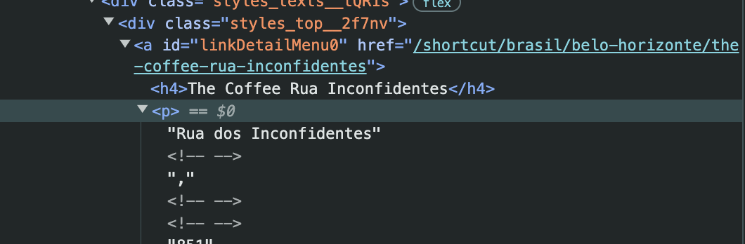
The data is extracted from The Coffee’s website. There is no single recipe or approach for webscraping: each website is organized differently, though there are patterns. In the case of The Coffee, units are separated by country and city; additionally each unit is identified by a name and has an address
The website
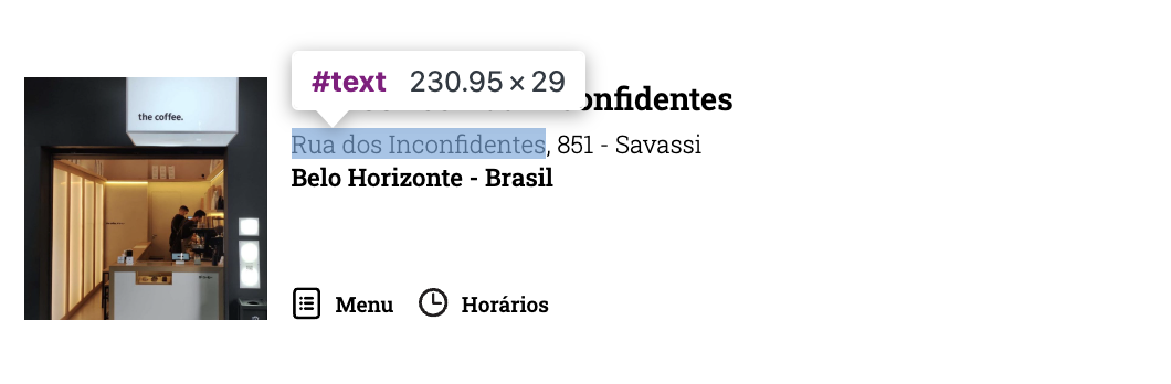
The site presents every unit by country and city. The print below shows an example unit in Belo Horizonte, Brazil.
Using R
The code below extracts the url related to every individual city in Brazil.
# Base url
base_url <- "https://thecoffee.jp/shortcut/brasil"
# Parse HTML
page_list_brazil <- xml2::read_html(base_url)

# Gets the urls for all cities in Brazil

page_list_cities <- page_list_brazil |>
  html_elements(xpath = "//div/ul/li/a") |>
  html_attr("href")

page_list_cities <- page_list_cities[str_detect(page_list_cities, "brasil/")]

url_cities <- str_c(base_url, str_remove(page_list_cities, "shortcut/brasil/"))
The code below is a function the scrapes the information of all shops for a given url of a city. The output is a simple data.frame.
scrape_the_coffee <- function(url) {

  # Parse the html
  page <- xml2::read_html(url)
  # Find the the name of the shop
  coffee_shop_name <- page |>
    rvest::html_elements(xpath = "//div/ul/li/div/div/a/h4") |>
    rvest::html_text()
  # Find the address of the shop
  address_list <- page |>
    rvest::html_elements(xpath = "//div/ul/li/div/div/a/p") |>
    rvest::html_text()
  # Remove shops that are not open yet
  address_list <- address_list[!str_detect(address_list, "coming soon")]
  street_name <- address_list[seq(1, length(address_list), 2)]
  city_name <- address_list[2]

  full_address <- paste(street_name, city_name)

  # Store results in a tibble
  out <- tibble::tibble(
    name = coffee_shop_name,
    address = full_address,
    street_name = street_name,
    city_name = city_name
  )

  return(out)

}
Functional approach
The simplest approach to implement this function is applying it over a vector with all urls for all cities. This means that the scrape_the_coffee function will be executed on each individual value of the url_cities text vector.
This approach is usually quicker and can be scaled with parallel processing (e.g. parallel::mclapply). Speed, however, usually isn’t a top priority with web scraping and can even be a detriment as it might lead to an excess number of requests.
It’s important to note that web scraping is liable to errors due to internet connection issues. As such it’s good practice to implement it in a error-prone fashion. The easiest way to do so in the functional approach is to wrap the function with purrr::safely. This way, errors don’t stop the function and are stored in a specific error class, making it easier to debug it afterwards.
# Scrape all cities

# Apply the scrape_the_coffee function over url_cities
safe_scrape_the_coffee <- safely(scrape_the_coffee)
coffee_locations <- map(url_cities, safe_scrape_the_coffee)
# Name the list for convinience
names(coffee_locations) <- url_cities
# Stack the results of the list into a single table
dat <- bind_rows(coffee_locations, .id = "url")
Loop approach
The code below shows how to implement the same procedure using a typical for-loop syntax. This approach is usually more intuitive and easier to follow. It’s generally better to use this approach in more complex web scrapping endeavors.
For illustration purposes, I show how to add a progress bar to the loop and a timeout.
# Define a progress bar
pb <- txtProgressBar(min = 1, max = length(url_cities), style = 3)
ls <- vector("list", length(url_cities))

for (i in seq_along(url_cities)) {

  # Get the current city
  url <- url_cities[i]
  current_city <- basename(url)
  message("Scraping data for: ", current_city)
  # Safely apply the scrape_the_coffee function
  ls[[i]] <- try(scrape_the_coffee(url))
  # Update progress bar
  setTxtProgressBar(pb, i)
  # Small timeout to avoid problems
  Sys.sleep(runif(1, min = 1, max = 5))

}
Cleaning the data
unnabreviate <- function() {
  c("Av\\." = "Avenida",
    "Al\\." = "Alameda",
    "R\\."  = "Rua",
    "Dr\\." = "Doutor",
    "Visc\\." = "Visconde",
    "Pres\\." = "Presidente",
    "Mal\\." = "Marechal")
}

dat <- dat |>
  mutate(
    city_name = str_remove(city_name, " - Brasil"),
    address = str_replace_all(address, unnabreviate()),
    country = "Brasil"
    )
Geocoding
Geocoding is the process of finding a street address based on a latitude/longitude pair or vice-versa. Typically, we need to call an external provider for this. In this case, I use the Google Maps API via the tidygeocoder package to find the corresponding lat/lng pair for each address.
# Geocode using Maps API
coffee <- tidygeocoder::geocode(
  dat,
  address = address,
  method = "google"
  )

# Convert to spatial data.frame
shops <- st_as_sf(
  coffee,
  coords = c("long", "lat"),
  crs = 4326,
  remove = FALSE
  )
Results
The table below shows the final results of the web scraping and geocoding process.
| City | # Shops | Share BR (%) |
|---|---|---|
| São Paulo | 53 | 26.50% |
| Curitiba | 29 | 14.50% |
| Brasília | 21 | 10.50% |
| Rio de Janeiro | 13 | 6.50% |
| Fortaleza | 10 | 5.00% |
| Porto Alegre | 9 | 4.50% |
| Florianópolis | 6 | 3.00% |
| Vitória | 5 | 2.50% |
| Campinas | 4 | 2.00% |
| Belo Horizonte | 3 | 1.50% |
leaflet(shops) %>%
  addTiles() %>%
  addMarkers(label = ~name) %>%
  addProviderTiles("CartoDB") %>%
  setView(lng = -46.65590, lat = -23.561197, zoom = 12)
Get Google Maps ratings
cur_shops <- filter(shops, city_name == "Curitiba")

get_ratings <- function(lat, lng) {

  location <- c(lat, lng)
  places <- google_places("The Coffee", location = location, radius = 10)
  res <- places$results

  subres <- res %>%
    unnest(cols = "geometry") %>%
    unnest(cols = "location") %>%
    select(
      business_status, name, formatted_address, rating, user_ratings_total,
      lat, lng
    )

}

ratings <- map2(cur_shops$lat, cur_shops$long, get_ratings)

dat_ratings <- ratings |>
  bind_rows() |>
  distinct() |>
  filter(str_detect(name, "^The Coffee"))

dat_ratings <- dat_ratings |>
  mutate(
    street_name = str_extract(formatted_address, "^[^,]+"),
    street_name = str_replace_all(street_name, unnabreviate()),
    street_name = stringi::stri_trans_general(street_name, "latin-ascii"),
    street_number = as.numeric(str_extract(formatted_address, "(?<=, )\\d+(?=\\b)"))
  )
Merging with Census information
The code below shows how to gather census tract data for each The Coffee shop. Census tracts are the smallest administrative division that present socioeconomic and demographic data.
Code
# Interpolation -------------------------------------------------------------

## Functions ---------------------------------------------------------------

# Creates a n minute walk isochrone around a point
get_buffer <- function(point, radius = 5, simplified = FALSE) {

  stopifnot(length(radius) == 1 && is.numeric(radius))

  if (simplified) {
    point |>
      sf::st_transform(crs = 31982) |>
      # Simplified assumption
      sf::st_buffer(dist = ((1.5 - 1.2) / 2 + 1.2) * 60 * radius)
  } else {
    point |>
      sf::st_transform(crs = 31982) |>
      osrm::osrmIsochrone(breaks = radius, osrm.profile = "foot") |>
      nngeo::st_remove_holes()
  }

}

# Interpolates an area with census tracts and aggregates population and households
interpolate_census <- function(census, target, variables = c("v0001", "v0003")) {

  if (st_crs(census) != st_crs(target)) {
    warning("CRS mismatch")

    census <- st_transform(census, crs = 31982)
    target <- st_transform(target, crs = 31982)

  }

  # Select variables
  census <- dplyr::select(census, dplyr::all_of(variables))
  # Interpolate areas
  interp <- st_interpolate_aw(census, target, extensive = TRUE)

  return(interp)

}

# Wrapper around get_buffer and interpolate_census
find_population <- function(shop, census, radius = 5, simplified = FALSE) {

  # Compute a 5-minute isochrone around
  buffer <- get_buffer(shop, radius, simplified)
  interpolated <- suppressWarnings(interpolate_census(census, buffer))

  return(interpolated)

}

## Interpolate -------------------------------------------------------------

# Uniquely identifies each shop
city_shops <- city_shops |>
  mutate(shop_id = row_number())

# To improve speed convert the full census data to 31982
city_census_utm <- st_transform(city_census, crs = 31982)

city_shops_census <- parallel::mclapply(
  split(city_shops, city_shops$shop_id),
  \(x) find_population(x, census = city_census_utm)
  )

city_shops_census <- bind_rows(city_shops_census, .id = "shop_id")

city_shops <- city_shops |>
  mutate(shop_id = as.character(shop_id)) |>
  left_join(st_drop_geometry(city_shops_census))
