# Setup -------------------------------------------------------------------
library(geobr)
library(dplyr)
library(ggplot2)
library(stringr)
library(sf)
library(ggnewscale)
library(showtext)
import::from(janitor, clean_names)
import::from(readxl, read_excel)
import::from(sidrar, get_sidra)
import::from(stringi, stri_trans_general)
import::from(tidyr, separate_wider_delim)
font_add_google("Lato", "Lato")
showtext_auto()
# Data --------------------------------------------------------------------
# Download data from SIDRA (Brazilian Institute of Geography and Statistics database)
# Table 9605: Population by race/color
sidra9605 <- get_sidra(9605, variable = 93, geo = "City")
url <- "https://geoftp.ibge.gov.br/organizacao_do_territorio/divisao_regional/divisao_regional_do_brasil/divisao_regional_do_brasil_em_regioes_geograficas_2017/tabelas/regioes_geograficas_composicao_por_municipios_2017_20180911.xlsx"
nmfile <- tempfile(fileext = "xlsx")
download.file(url, nmfile)
dim_inter <- readxl::read_excel(nmfile)
dim_inter <- dim_inter |>
rename(
code_muni = CD_GEOCODI,
code_intermediate = cod_rgint,
code_immediate = cod_rgi,
name_muni = nome_mun,
name_intermediate = nome_rgi
) |>
mutate(across(starts_with("code"), as.numeric))
# Helper function to standardize text: remove accents and convert to lowercase
str_simplify <- function(x) {
y <- stringi::stri_trans_general(x, "latin-ascii")
y <- stringr::str_to_lower(y)
return(y)
}
pop <- sidra9605 |>
as_tibble() |>
janitor::clean_names() |>
mutate(
code_muni = municipio_codigo,
code_region = str_sub(code_muni, 1, 1),
code_state = str_sub(code_muni, 1, 2),
race = str_simplify(cor_ou_raca),
race_label = cor_ou_raca,
pop = valor
) |>
mutate(across(starts_with("code"), as.numeric))
pop <- left_join(
pop,
select(dim_inter, code_muni, code_intermediate, code_immediate),
by = "code_muni"
)
pop <- pop |>
# Split municipality name and state abbreviation
separate_wider_delim(
cols = municipio,
delim = " - ",
names = c("name_muni", "abbrev_state")
) |>
# Select and reorder relevant columns
select(starts_with("code"), name_muni, abbrev_state, race, race_label, pop) |>
# Remove totals and calculate proportions by municipality
filter(race != "total") |>
mutate(prop = pop / sum(pop, na.rm = TRUE), .by = "code_muni")
# Define grouping variables for different geographic levels (id variables)
pop_summary <- list(
region = c("code_region"),
state = c("code_state"),
intermediate = c("code_intermediate"),
immediate = c("code_immediate"),
brasil = c("race")
)
# Function to create summary tables
summarise_tables <- function(x) {
pop |>
# Sums population by id variables + race
summarise(
total = sum(pop, na.rm = TRUE),
.by = c(all_of(x), "race", "race_label")
) |>
# Computes population shares by id variables
mutate(
prop = total / sum(total),
.by = all_of(x)
)
}
# Create all summary tables at once
tbls <- lapply(pop_summary, summarise_tables)
# Find the highest share within each intermediate region
top_inter <- tbls$intermediate |>
group_by(code_intermediate) |>
slice_max(prop, n = 1) |>
ungroup()
geo_inter_full <- read_intermediate_region(showProgress = FALSE, simplified = FALSE)
geo_inter <- read_intermediate_region(showProgress = FALSE)
geo_inter_full <- left_join(geo_inter_full, top_inter, by = "code_intermediate")
inter <- left_join(geo_inter, top_inter, by = "code_intermediate")
# Map ---------------------------------------------------------------------
legend_breaks <- seq(0.5, 0.8, 0.1)
legend_labels <- legend_breaks * 100
legend_limits <- c(0.4, 0.85)
base_map <- ggplot() +
geom_sf(
data = filter(inter, race != "branca"),
aes(fill = prop),
lwd = 0.1,
color = "white"
) +
scale_fill_distiller(
name = "% Pardos",
palette = "Purples",
direction = 1,
breaks = legend_breaks,
labels = legend_labels,
limits = legend_limits
) +
# Creates a secondary scale using ggnewscale::new_scale_fill
new_scale_fill() +
geom_sf(
data = filter(inter, race == "branca"),
aes(fill = prop),
lwd = 0.1,
color = "white"
) +
scale_fill_distiller(
name = "% Brancos",
palette = "Greens",
direction = 1,
breaks = legend_breaks,
labels = legend_labels,
limits = legend_limits
)
# Find the region with the highest share for each race
sf_top <- inter |>
group_by(race) |>
slice_max(prop, n = 1, na_rm = TRUE) |>
ungroup()
# Get the position of the centroids (for the arrow)
coords_centroid_top <- sf_top |>
st_centroid() |>
st_coordinates()
# Auxiliar data.frame to position the text labels
df_annotation <- tibble(
x = c(-40, -65, -43, -44),
y = c(-27, -18, -32, 2),
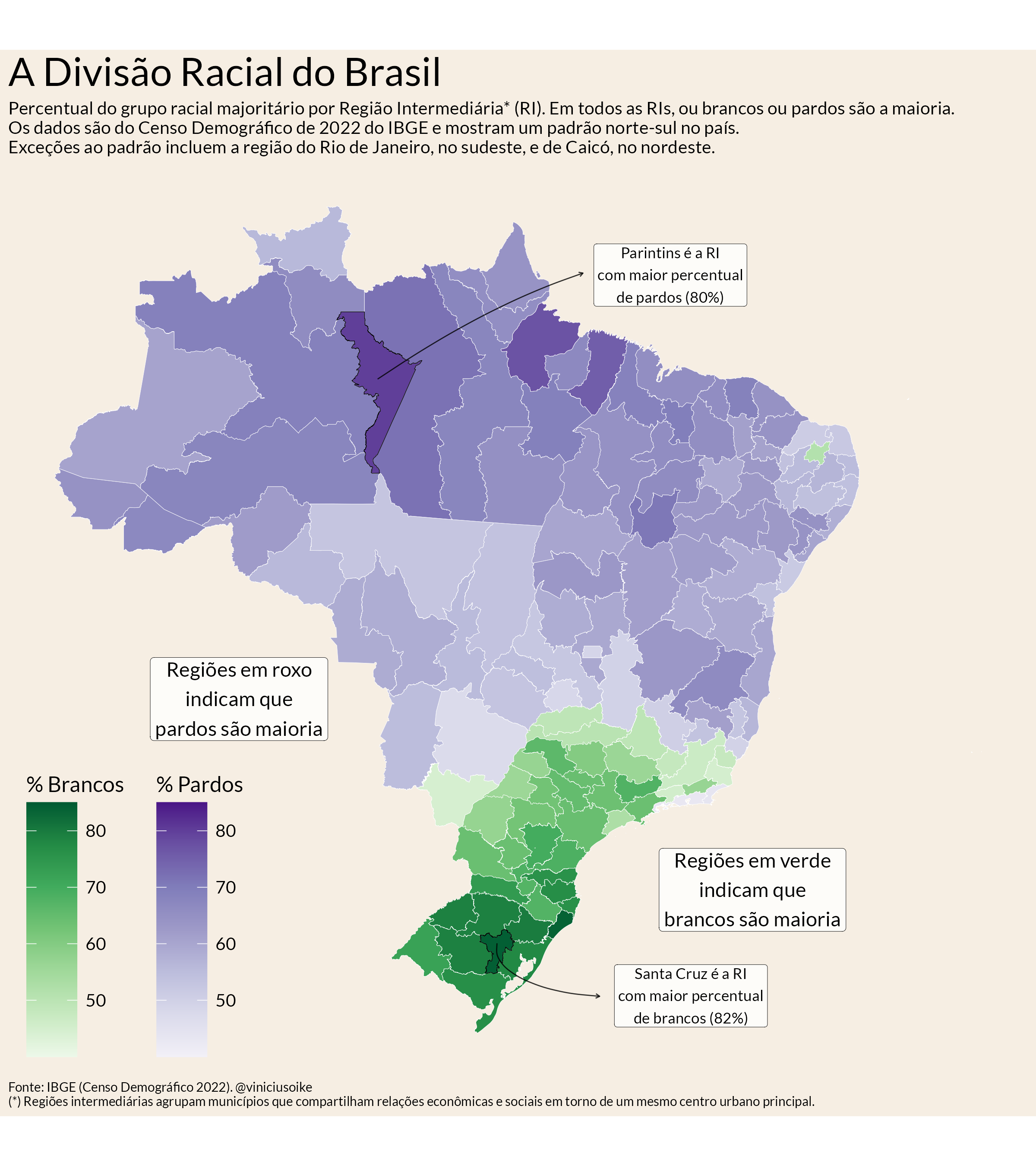
label = c(
"Regiões em verde\nindicam que\nbrancos são maioria",
"Regiões em roxo\nindicam que\npardos são maioria",
"Santa Cruz é a RI\ncom maior percentual\nde brancos (82%)",
"Parintins é a RI\ncom maior percentual\nde pardos (80%)"
)
)
# Add text labels to plot
map_annotations <- base_map +
geom_label(
data = df_annotation,
aes(x = x, y = y, label = label),
family = "Lato",
size = c(4, 4, 3, 3),
fill = "white", # background color
alpha = 0.8, # transparency
label.padding = unit(0.2, "lines"), # padding around text
label.size = 0.1 # border thickness
) +
# Top %share -- Santa Cruz - Lajeado | Parintins-- dark border
geom_sf(
data = filter(inter, code_intermediate %in% c(1304, 4308)),
fill = NA,
color = "black",
lwd = 0.15
) +
# arrow/curve segment: Santa Cruz - Lajeado
geom_curve(
data = data.frame(x = coords_centroid_top[1, 1], y = coords_centroid_top[1, 2]),
aes(x = x, y = y + 0.25, xend = x + 5, yend = y - 2.25),
linewidth = 0.3,
angle = 45,
alpha = 0.8,
arrow = arrow(length = unit(2.5, "pt"))
) +
# arrow/curve segment: Parintins
geom_curve(
data = data.frame(x = coords_centroid_top[2, 1], y = coords_centroid_top[2, 2]),
aes(x = x, y = y, xend = x + 10, yend = y + 5),
linewidth = 0.3,
angle = 45,
curvature = -0.1,
alpha = 0.8,
arrow = arrow(length = unit(2.5, "pt"))
) +
# Remove excess white space from map
coord_sf(xlim = c(-72.2, -35.5))
# Add title and thematic elements
final_map <- map_annotations +
labs(
title = "A Divisão Racial do Brasil",
subtitle = "Percentual do grupo racial majoritário por Região Intermediária* (RI). Em todos as RIs, ou brancos ou pardos são a maioria.\nOs dados são do Censo Demográfico de 2022 do IBGE e mostram um padrão norte-sul no país.\nExceções ao padrão incluem a região do Rio de Janeiro, no sudeste, e de Caicó, no nordeste.",
caption = "Fonte: IBGE (Censo Demográfico 2022). @viniciusoike\n(*) Regiões intermediárias agrupam municípios que compartilham relações econômicas e sociais em torno de um mesmo centro urbano principal.") +
ggthemes::theme_map(base_family = "Lato") +
theme(
plot.title = element_text(
hjust = 0,
size = 22
),
plot.subtitle = element_text(
hjust = 0,
size = 10
),
plot.caption = element_text(hjust = 0),
legend.position = "inside",
legend.position.inside = c(0.01, 0.01),
legend.box = "horizontal",
legend.key.size = unit(1, "cm"),
legend.text = element_text(size = 10),
legend.title = element_text(size = 12),
plot.background = element_rect(fill = "#F6EEE3", color = "#F6EEE3"),
legend.background = element_rect(fill = "#F6EEE3", color = "#F6EEE3")
)
ggsave(
here::here("static/images/censo_mapa_raca.svg"),
final_map,
width = 8,
height = 9
)